Direct volume rendering is a powerful technique for visualizing the structure of volume datasets. As devices for the acquisition of volume data are created and improved upon, the applications of direct volume rendering are growing from medicine and computational fluid dynamics to include astronomy, physics, meteorology, and geology. The most attractive aspect of direct volume rendering is actually its defining characteristic: it maps directly from the dataset to a rendered image without any intermediate geometric calculations. This is in contrast to traditional isosurface rendering, where the rendering step is proceeded by the calculation of an isosurface for a particular data value. Direct volume rendering can also avoid the time-consuming processes of segmentation and classification, because visualization can be done without any high-level information about the material content at each voxel.
Direct volume rendering is based on the premise that the data values in the volume are themselves a sufficient basis for creating an informative image. What makes this possible is a mapping from the numbers which comprise the dataset to the optical properties that compose a rendered image, such as opacity and color. This critical role is performed by the transfer function. Because the transfer function is central to the direct volume rendering process, picking a transfer function appropriate for the dataset is essential to creating an informative, high-quality rendering.
The most general transfer functions are those that assign opacity, color, and emittance [LCN98]. However, much direct volume rendering uses transfer functions assigning only an opacity, with the color and intensity derived from simulated lights which illuminate the volume. For the purposes of this thesis, the term opacity functions is used to refer to this limited subset of transfer functions. Once the opacity function has been applied to the volume, the surfaces of the opaque regions are then shaded according to a simple shading model, such as the Phong model [Pho75]. Although this thesis explores opacity functions only, its results would be helpful in creating more general types of transfer functions as well.
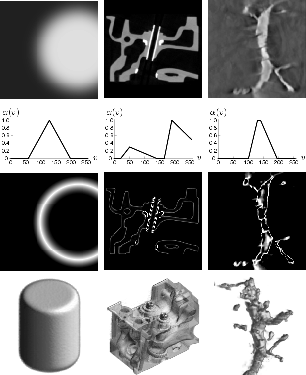 |
In order to gain some intuition about the role opacity functions play in visualizing the structure of a volume dataset, it helps to look at opacity functions applied to two dimensional slices of sample datasets. Figure 1.1 shows the process for three datasets, with (from top to bottom) a slice of the dataset, a plot of the opacity function, the result of applying the opacity function to the slice, and an image rendered using the shown opacity function. The dataset analyzed in the left column is a synthetic dataset of a cylinder, which will be used repeatedly for illustrative purposes. In the middle column is a computed tomography (CT) scan of an engine block1. The last column shows one of the neuron datasets from the Collaboratory for Microscopic Digital Anatomy (CMDA), in which the Program of Computer Graphics is a research participant [EGLea96]. The neuron data was tomographically generated from a sequence of transmission electron microscopy (EM) images2.
Note that in each of these cases, the primary purpose of the opacity functions is to make opaque those values that occur around the boundaries of objects. This allows the shape of the objects to be seen in the rendered image without being obscured by the surrounding medium. If the opacity function makes these boundaries partially transparent, we can look through outer surfaces in the object (such as the engine block) to see internal structure. Since the opacity function is applied to the whole volume in a position-independent way, volume rendering relies on the premise that the interesting structural components of the volume, such as boundaries, have a reliable correlation with data value. If this is the case, then there should be an opacity function which produces an informative rendering.
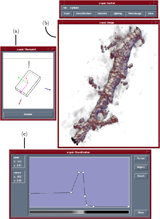 |
The tools used to find opacity functions and render images might look something like Figure 1.2, which shows the direct volume rendering interface that was built for the CMDA project3. The user sets the viewpoint in window (a), which provides feedback with a wireframe box indicating the orientation and aspect ratio of the volume. The rendered image appears in window (b). Not shown are the interface for setting the position and color of the lights, and a tool for inspecting two dimensional slices of the data. The tool used to set the opacity function is shown in window (c). The user sets the number and location of control points which define an opacity function as a series of linear ramps.
In practice, a frustrating amount of time is spent adjusting the location of these points to make the image look ``right''. The general problem of transfer function specification is very difficult, but even simply finding a good opacity function is challenging. To make a high-quality rendering, an opacity function must satisfy at least two guidelines:
Unfortunately, satisfying these constraints is an unintuitive task. Users looking at slices of the dataset can easily spatially locate features of interest, but finding data values which consistently correspond to the features of interest throughout the volume is not straight-forward. The second guideline is related to the fact that every direct volume rendering technique has strengths and weaknesses, and poorly designed opacity functions can reveal the weaknesses. Again, the selection of opacity functions is not intuitive, so typically the user searches for an opacity function by trial and error, adjusting it and repeatedly re-rendering to see the effects on the rendered output.