Direct volume rendering of boundaries

The question could be asked- ``If the goal is to render the boundaries of objects, why is direct volume rendering being used, as opposed to isosurface rendering?'' The standard argument for direct volume rendering as opposed to isosurface rendering is that in the former, ``every voxel contributes to the final image'', while in the isosurface rendering, only a small fraction of voxels (those containing the isovalue) contribute to the final image [Lev88]. This argument is not very convincing, since there is no consistent correlation between the quality of the image and the number of voxels contributing to its formation. Too many opaque voxels result in a cloudy image, or an image where an interesting portion of the structure is unintentionally obscured. It is just as important that the transfer function leave some parts of the volume transparent as it is that it make the interesting parts opaque; otherwise the volume rendered image would provide no additional insight into the structure of the volume.

The basic benefit of direct volume rendering over isosurface rendering is that it provides much greater flexibility in determining how the voxels contribute to the final image. Voxels over a range of values can all contribute to the image, with varying amounts of importance, depending on the transfer function. Also, while an isosurface can only show structure based solely on data value, the transfer function can do so based on other quantities as well, such as gradient magnitude.

This motivates why direct volume rendering can be used in situations where the structure of the data is amorphous, as in gaseous simulations [Max95]. More importantly, it motivates the use of direct volume rendering in medical imaging situations where there noise or measurement artifacts distort the isosurfaces away from the shape of the object boundary. To the extent that the objects' surfaces are associated with a range of values, the transfer function for direct volume rendering can make a range of values opaque or translucent.

Figure 1.3: Slice of neuron in tomographic plane. Artifacts from the lack of projection data at some angles are visible as the bright spots on either side of the dendrite, as well as the light streaks.

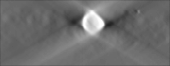As an example to exhibit the usefulness of direct volume rendering versus isosurface rendering, consider some neuron data from the CMDA project. Figure 1.3 shows a slice of a spiny dendrite dataset. Note the dark regions on either side of the neuron, and the light streaks which emanate from its top and bottom. These are artifacts from the tomographic process which reconstructs three dimensional information from a series of two dimensional projections. Because there are ranges of angles in which projection data cannot be obtained, there are orientations for which the quality of the tomographic reconstruction is poor, causing the surface of the neuron to be blurred or distorted. A further difficulty is the fact that the radio-opaque dye which renders the neuron visible is sometimes absorbed unevenly.

Figure 1.4: Comparison of volume rendering methods

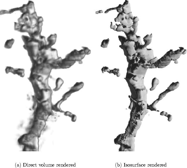Fig. 1.4 shows two renderings of a mammalian neuron dataset, using the same viewing angle, shading, and lighting parameters, but rendered with different algorithms: a shear-warp direct volume rendering produced with the Stanford VolPack rendering library[LL94] and a non-polygonal ray-cast isosurface rendering. Towards the bottom of the direct volume rendered image, there is some fogginess surrounding the surface, and the surface itself is not very clear. As can be confirmed by looking directly at slices of the raw data, this corresponds exactly to a region of the dataset where the material boundary is in fact poorly defined. The surface rendering, however, shows as distinct a surface here as everywhere else, and in this case the poor surface definition in the data is manifested as a region of rough texture. This can be misleading, as there is no way to know from this rendering alone that the rough texture is due to measurement artifacts, and not a feature on the dendrite itself.