Comparison with Levoy's two dimensional opacity functions

The main result of Levoy's influential paper, ``Display of Surfaces from Volume Data''[Lev88], was to demonstrate the usefulness of volume rendering for what might otherwise be considered the domain of isosurface rendering-- the visualization of surfaces in regularly sampled volume data. He demonstrated that not only is direct volume rendering appropriate for this task, but that in some aspects it is superior to isosurface rendering. It avoids the explicit creation of a surface geometry, and it displays ambiguous or under-sampled features as ``faint wisps'', a more accurate representation than that given by isosurfacing. His success can be attributed to the careful design of the opacity functions which he developed for the two visualization tasks described in his paper. Because there are many similarities between the goals addressed in Levoy's paper and in this thesis, we review the opacity functions which Levoy designed and the visualization problems which motivated them. We conclude the chapter with some observations about the differences between Levoy's methods and the ones advanced in this thesis.

Visualizing isosurfaces in smoothly varying data

Levoy's first task was visualizing isosurfaces of electron density functions. These datasets are characterized by smooth and slow variations of the data value throughout the volume.

Figure 5.10: Slices of electron density dataset

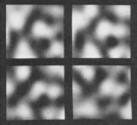
From the four sample cross-sections of such a dataset shown in Figure 5.10 (taken from Levoy's paper), we can see that these datasets do not exhibit any of the characteristics assumed for this thesis. There are no regions of relatively constant value contained by boundary regions where the data value changes quickly. The discontinuities which exist with material boundaries are not present in electron density functions. Still, it is important to review the opacity function Levoy developed for this type of data because it is the only style of two dimensional opacity function which has since received any significant attention in the volume rendering literature[Mur95,YESK95,LCN98]. Also, the opacity function he designed for this application has proven to have utility for a wider variety of datasets.

Because Levoy uses volume rendering instead of true isosurface extraction to visualize the isovalue contours, the rendered surfaces will necessary have some thickness. Levoy states that the ``most pleasing image'' results from making the isosurface appear to have equal thickness everywhere. One way to achieve this is with a opacity function which takes into account the gradient of the data value. Specifically, if we assume that the data value varies linearly with position near the isosurface, then the range of values which needs to be made opaque is proportional to the magnitude of the gradient. When the data value changes quickly as a function of position, a wider range of values need to be made opaque so as to create an opaque region of fixed thickness, and conversely low rates of change in data value require opacity for a narrower ranges of values. The plot of the two dimensional opacity function which achieves this is shown in Figure 5.11(a), a diagram taken from Levoy's paper. Also, to facilitate comparison with the gray-scale graphical representation of the two dimensional opacity functions presented in this thesis, a gray-scale representation of Levoy's function is shown in Figure 5.11(b). We continue the convention used in Chapter 5, letting $v = f(\mathbf{x})$ and $g = \vert\nabla f(\mathbf{x})\vert$, though Levoy's figures employ a slightly more complicated notation.

Figure 5.11: Levoy's opacity function for isovalue surfaces. In (a), a three dimensional plot of the function, from Levoy's paper. The data value axis extends to the lower right, and the gradient magnitude axis extends to the upper right, with opacity on the vertical axis. In (b), a gray scale representation of the same function. In (a), the isovalue is notated $f_v$, while in (b) it is notated $v_0$.

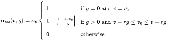
There are three degrees of freedom in this type of opacity function which need to be defined before stating its formula:

• $v_0$: the isovalue around which the opacity will be assigned (Levoy refers to this quantity as $f_v$)
• $r$: the desired thickness of the isosurface, in units of voxel edge length
• $\alpha _0$: the maximum opacity of the isosurface (notated $\alpha _v$ by Levoy)

Strictly speaking, Levoy defines his opacity as a function of position $\mathbf{x}$ within the volume, but the terms which appear in his formula are the data value at $\mathbf{x}$, $v = f(\mathbf{x})$, and the gradient magnitude at $\mathbf{x}$, $g = \vert\nabla f(\mathbf{x})\vert$. Thus the opacity function can be expressed as:

$$\alpha _{iso}(v,g) = \alpha _0 \left\{ \begin{array}{ll} 1 & \mbo... ...\leq v_0 \leq v + rg$} \end{array} \\ 0 & \mbox{otherwise} \end{array} \right.$$ (19)

It is the second line of Equation 5.14 which establishes the proportionality between the gradient magnitude and the range of data values which are assigned opacity. This in turn creates the ``V'' shape of the opaque region in $(v,g)$ space, flaring linearly with gradient magnitude (Figure 5.11)

Visualizing region boundary surfaces

The second visualization task addressed in Levoy's paper is the rendering of ``region boundary surfaces'' in the specific context of CT medical imaging technology. Like the visualization task discussed in this thesis, Levoy's goal is to visualize the interfaces between adjacent regions of uniform material. However, since Levoy restricts himself to the domain of CT datasets, he makes strong assumptions about the spatial inter-relationship between the material regions. Quoting from this paper:

``We assume that scenes contain an arbitrary number of tissue types bearing CT numbers falling within a small neighborhood of some known value. We further assume that tissues of each type touch tissues of at most two other types in a given scene. Finally, we assume that, if we order the types by CT number, then each type touches only types adjacent to it in the ordering.''

To characterize the opacity function Levoy developed for this case, we notate the ``CT numbers'' (the materials' data values in the CT scan) as $v_i$, where each material is tagged with an integer $i$. Next, an opacity $\alpha _i$ is assigned to material $i$ so that the various materials can be visually differentiated in the rendering. Values which fall between the known material values $v_i$ and $v_{i+1}$ are assigned an opacity by linearly interpolating between $\alpha _i$ and $\alpha _{i+1}$. Finally, and most importantly, to accentuate the boundaries between the regions, the opacity is scaled by the gradient magnitude. Figure 5.12(a) shows the plot of the opacity function which appeared in Levoy's paper, and Figure 5.12(b) shows the gray-scale representation.

Figure 5.12: Levoy's opacity function for region boundary surfaces. In (a), a three dimensional plot of the function, using the same axes as in Figure 5.11(a). In (b), a gray scale representation of the function. The three known material values are labeled $f_{v_A}$, $f_{v_B}$, and $f_{v_C}$ in (a), while in (b) they are notated simply $v_A$, $v_B$, and $v_C$. Similarly, the material opacities $\alpha _{v_A}$, $\alpha _{v_B}$, $\alpha _{v_C}$ in (a) are notated $\alpha _A$, $\alpha _B$, and $\alpha _C$ in (b).

The final opacity function is then:

$$\alpha _{bound}(v,g) = g \left\{ \begin{array}{ll} \alpha _{i+1} ... ...mbox{if $v_i \leq v \leq v_{i+1}$} \\ 0 & \mbox{otherwise} \end{array} \right.$$ (20)

In comparing our method with the second of Levoy's two opacity functions, it should be stressed that he assumes the CT numbers $v_i$ are known for each type of biological material. This thesis, however, aims to be more general and require less prior knowledge. Because the opacity function generation presented in this thesis is grounded in the measured properties of the data, the user is (ideally) freed from setting material data values by hand. Levoy is nonetheless justified in making his assumption, because in medical imaging situations where CT is being used, there is a high degree of consistency between scans in the data values which arise from human tissue types.

The assumption about having a strict progression of nested regions with increasing data values is stronger than any assumption made in this thesis. For instance, the nested cylindrical shells in Section 5.3 violate Levoy's assumption but are well handled by our method for two dimensional opacity function generation. On the other hand, this thesis makes the strong assumption that all boundaries have the same thickness. Levoy makes no assumptions whatsoever about the the thickness of boundaries, nor does he rely on any particular boundary model for defining the opacity function. He simply requires that the boundary region have higher gradient magnitude that the material interior, so that scaling the opacity by the gradient magnitude (Equation 5.15) causes material interiors to be suppressed in the rendering.