Implementation

Before we can create histogram volumes, there are several implementation issues that need to be resolved, starting with the spatial resolution of the grid on which we sample $f$, $f'$, and $f''$ throughout the volume. If the grid is too sparse, we risk missing the boundary. Instead of having a dense and continuous distribution of ``hits'' in the histogram volume, we would have only sparse or broken coverage of the curves we are looking for. If the grid is too dense, we have excess computation.

The approach taken in this thesis is to measure $f$, $f'$, and $f''$ exactly once per voxel, at the original sample points of the dataset. There are two reasons for this. First is ease of computation. Because we are working only with the original data points of the volume, there is no need to perform reconstruction to measure $f$, and the measurements of $f'$ and $f''$ are greatly facilitated by the use of masks, a computational tool to measure properties of discrete data. These will be explained shortly. Second, because bandlimiting ensures that there is always some boundary blurring, and because the boundaries of real objects are apt to assume a variety of positions and orientations relative to the sampling grid, sampling over the whole dataset will insure that the sample points fall at a variety of positions within the boundary region, leading to more complete coverage of the curves in the scatterplots and histogram volume. Of course, the more bandlimiting there is, the more blurred the boundaries will be, leading to a greater accumulation of hits along the curves in the histogram volume and in the scatterplots. A more mathematical treatment of this relationship is given in Appendix A.

The remaining implementation issues of histogram volume creation are unfortunately matters of parameter setting. Though the goal of this research is to reduce the total number of parameters that need to be adjusted before informative renderings can be achieved, there are in fact a few input parameters necessary for the creation of the histogram volume itself. This is why the generation of transfer functions is (at best) semi-automatic.

One variable in the histogram volume creation is the histogram resolution, that is, how many bins to use. The trade-off here is between the large storage and processing requirements caused by having many bins, and the inability to resolve patterns in the histogram volume caused by having too few. In our experiments, good results have been obtained with histogram volumes of sizes between $80^3$ and $256^3$, though there is no reason that the histogram volumes need to have equal resolution on each axis. In general, better results have been obtained from using larger histogram volumes. While a $256^3$ volume does not represent an exceedingly large storage or computational challenge to modern systems, the ability to get decent results from, for instance, a $128^3$ histogram volume, with the associated nearly 8-fold speed increase, makes the use of smaller histogram volumes an attractive alternative. A brief comparison of results from using different size histogram volumes is given in Chapter 6.

A more significant issue is the the range of values that each axis of the histogram volume should represent. Obviously along the data value axis, we should include the full range, since we want to capture all the values at which boundaries might occur. But along the axes for the first and second derivatives, it may make sense to include something less than the full range. This is because derivative measures are by nature very sensitive to noise, and thus will take on very high (or very low) values wherever noise occurs. If significant noise is present in the volume data, and if we included the full range of derivative values in the histogram volume, then the important and meaningful sub-range of derivative values might be compressed to a relatively small number of bins. This would hamper the later step of detecting patterns in the histogram volume. Of course, we have no a priori way of knowing what the meaningful ranges of derivatives values are. Currently, the derivative value ranges are set by hand, and this is a subject in need of further research.

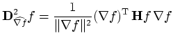
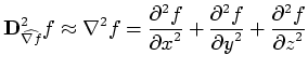
The most significant implementation issue is the method of measuring the first and second directional derivatives. The first derivative is actually just the gradient magnitude. From vector calculus [MT96] we have:

$$\mathbf{D}_\mathbf{v}f = \nabla f \cdot \mathbf{v},$$ (1)

thus

$$\mathbf{D}_{\widehat{\nabla f}}f = \nabla f \cdot \widehat{\nabla f} = \nabla f \cdot \frac{\nabla f}{\Vert\nabla f\Vert} = \Vert\nabla f\Vert.$$ (2)

Unfortunately there is no similarly compact formula for $\mathbf{D}^{2}_{\widehat{\nabla f}}f$, the second directional derivative along the gradient direction. Twice applying Equation 4.2 gives:

$$\mathbf{D}^{2}_{\widehat{\nabla f}}f = \mathbf{D}_{\widehat{\nabla f}}(\Vert\nabla f\Vert) = \nabla (\Vert\nabla f\Vert) \cdot \widehat{\nabla f} \nonumber$$

$$= \frac{1}{\Vert\nabla f\Vert} \nabla (\Vert\nabla f\Vert) \cdot \nabla f$$ (3)

Or, using the Taylor expansion of $f$ along $\widehat{\nabla f}$ [Fau93] gives:

$$\mathbf{D}^2_{\widehat{\nabla f}}f = \frac{1}{\Vert\nabla f\Vert^2} (\nabla f)^{\mathrm T} \, \mathbf{H} f \, \nabla f$$ (4)

where $\mathbf{H} f$ is the Hessian of $f$, a $3 \times 3$ matrix of second partial derivatives of $f$ [MT96]. Alternatively, we can use the Laplacian $\nabla^{2} f$ to approximate $\mathbf{D}^{2}_{\widehat{\nabla f}}f$:

$$\mathbf{D}^{2}_{\widehat{\nabla f}}f \approx \nabla^{2} f = \frac... ...rac{\partial^{2} f}{{\partial y}^{2}} + \frac{\partial^{2} f}{{\partial z}^{2}}$$ (5)

The approximation is exact only where the isosurfaces have zero mean surface curvature [Fau93].

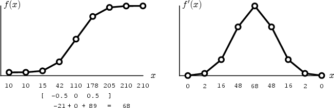
As all these derivative measures require taking first or second partial derivatives of the data along the axial directions, we need to develop masks which can measure these quantities. Masks are vectors of scalar weights, designed to measure certain properties of sampled data. The mask is centered at the sample point of interest, and the products between corresponding mask weights and sample values are summed to produce the final measurement. The combination of weights in the mask determine its functionality. As a simple example, Figure 4.3 demonstrates a mask ( $[-0.5~~0~~0.5]$) which measures the first derivative of one dimensional data.

Figure 4.3: Using a mask to measure first derivative. The data values $42$, $110$, and $178$ are multiplied by the mask values $-0.5$, 0, and $0.5$ respectively, and the products are summed to produce the final measurement.

Derivative measurement with this mask is called central differencing and is very commonly used in image processing[GW93]. Appendix B describes how central differences can be generalized to measure first and second partial derivatives in three dimensions.

Even though we have a way of measuring all the necessary partial derivatives in the volume, we still need to chose among the different measurement approaches for $\mathbf{D}^{2}_{\widehat{\nabla f}}f$. Each of the three expressions for $\mathbf{D}^{2}_{\widehat{\nabla f}}f$ given above suggest different implementations. While the Hessian method (Equation 4.4) has been found to be the most numerically accurate, the others have proven sufficiently accurate in practice to make them appealing by virtue of their computation efficiency. The Laplacian (Equation 4.5) computation is direct and inexpensive, but the most sensitive to quantization noise. The gradient of the gradient magnitude (Equation 4.3) is better, and its computational expense is lessened if the gradient magnitude has already been computed everywhere for the sake of volume rendering (e.g., as part of shading calculations). A more thorough characterization of the different second derivative measures is given in Appendix C. Deciding which derivative measures to use is the final parameter for histogram volume creation.

We can now give an algorithm for histogram volume creation:

• Initialize the histogram volume to all zero values.
• Make one pass through the volume looking for the highest values of $f'$ and $f''$, and the lowest value of $f''$. (Assume zero for the lowest value of $f'$). Set ranges on the histogram volume axes accordingly.
• Make a second pass through the volume:
  • Measure $f$, $f'$, and $f''$ at each sample point,
  • Determine which bin in the histogram volume corresponds to the measured combination of $f$, $f'$, and $f''$, and
  • Increment the bin's value.