Bandlimiting and thickness in terms of $\sigma$

Our goal here is to show the relationship between the boundary's frequency content and its thickness, and how this relationship effects our ability to record the presence of the boundary in the histogram volume. The Fourier transform is an important part of this analysis, and because there are variety of possible definitions for the transform, we state the particular definitions being used here:

$$F(\omega ) = \mathcal{F}(f)(\omega ) \equiv \int_{-\infty}^{\infty}f(x) e^{-i\omega x}~dx$$ (22)

$$f(x) = \mathcal{F}^{-1}(F)(x) \equiv \frac{1}{2\pi} \int_{-\infty}^{\infty}F(\omega ) e^{i\omega x}~d\omega$$ (23)

We will use the following to model the data value as a function of position within a boundary region:

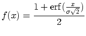$$f(x) = \frac{1+\operatorname{erf}(\frac{x}{\sigma \sqrt{2}})}{2}$$ (24)

Recall from Section 5.2 that the ``thickness'' of a boundary is defined to be $2\sigma$. Setting $v_{min} = 0$ and $v_{max} = 1$ in the the formula for $f(x)$ given in Section 5.1 produces Equation A.3. Any other values for the variables $v_{min}$ and $v_{max}$ represent some scaling or shifting of the boundary, and the Fourier transform is not meaningfully changed by these operations.

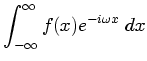
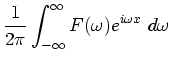
To find the Fourier transform of the $f(x)$ given above, we could simply apply the definition of the Fourier transform to $f(x)$, and then reduce the resulting expression. We can avoid this labor, however, by exploiting a useful property of the transform under integration, expressed here with $~\overset{\mathcal{F}}{\longleftrightarrow}~$ pointing to the two expressions which are transforms of each other:

$$g(x) ~\overset{\mathcal{F}}{\longleftrightarrow}~G(\omega ) ~\Rig... ...}}{\longleftrightarrow}~\frac{G(\omega )}{i\omega } + \pi G(0) \delta (\omega )$$ (25)

This states, in terms of a function $g(x)$ and its Fourier transform $G(\omega )$, how to find the transform of an integral if we already know the transform of the function being integrated. Aside from a ``DC'' term $\pi G(0) \delta (\omega )$ (which we will henceforth ignore¹⁸), when we integrate a function, the corresponding transform is divided by $i\omega$. We will use Equation A.4 to find the transform of $f(x)$ because doing so will bring us directly in contact with the attenuation in frequency space caused by the bandlimiting inherent in the measurement.

In order to exploit the property expressed in Equation A.4, we find the derivative of $f(x)$:

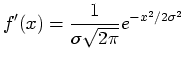$$f'(x) = \frac{1}{\sigma \sqrt{2\pi}} e^{-x^2/2\sigma ^2}$$ (26)

By our choice of $f(x)$, $f'(x)$ is a normalized Gaussian function with standard deviation $\sigma$. Its Fourier transform is[KK68]:

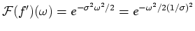$$\mathcal{F}(f')(\omega ) = e^{-\sigma ^2 \omega ^2/2} = e^{-\omega ^2/2(1/\sigma )^2}$$ (27)

Thus the transform of a Gaussian function is another Gaussian function, and there is an exact reciprocal relationship between their standard deviations. While the standard deviation in $f'(x)$ is $\sigma$, in $\mathcal{F}(f')(\omega )$ it is $1/\sigma$. Having $f'(x)$ and its transform $\mathcal{F}(f')(\omega )$, we can now use Equation A.4 to state the transform of the measured boundary function:

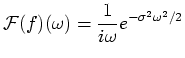$$\mathcal{F}(f)(\omega ) = \frac{1}{i\omega } e^{-\sigma ^2 \omega ^2/2}$$ (28)

It is possible to utilize the same process to find the transform of the un-blurred boundary function, which represents the boundary prior to the measurement process. This is the so-called Heaviside step function $h(x)$:

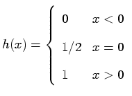$$h(x) = \left\{ \begin{array}{ll} 0 & \mbox{$x < 0$} \\ 1/2 & \mbox{$x = 0$} \\ 1 & \mbox{$x > 0$} \end{array} \right.$$ (29)

By definition, the derivative of the step function is the delta function $\delta (x)$. The Fourier transform of the delta function is trivial to compute:

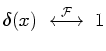$$\delta (x) ~\overset{\mathcal{F}}{\longleftrightarrow}~1$$ (30)

Then by again using Equation A.4 we can find the transform of the step function:

$$h(x) ~\overset{\mathcal{F}}{\longleftrightarrow}~\frac{1}{i\omega }$$ (31)

Since we know from Fourier theory that the spectrum of the convolution of two functions is exactly the product of the two functions' spectra, we see from the expression for $\mathcal{F}(f)(\omega )$ (Equation A.7) that the spectrum of the measured boundary is the product of the spectrum of the step function ($1/i\omega$) times a Gaussian function $e^{-\sigma ^2 \omega ^2/2}$. Thus, $e^{-\sigma ^2 \omega ^2/2}$ is precisely the attenuation in frequency caused by the bandlimiting in the measurement process. We can now state the relationship between measured boundary thickness and bandlimiting:

The boundary thickness will be $2\sigma$ when the bandlimiting due to measurement is equivalent to multiplication in frequency space by a Gaussian function with standard deviation $1/\sigma$.

Footnotes

... ignore¹⁸

The DC (direct current) component of the Fourier transform represents the average value of the function. Since all the relevant characteristics of the boundary's Fourier transform are in terms of non-zero frequencies, the DC component is not important for this analysis.