Mathematical boundary analysis

In order to develop a method for opacity function generation that uses our boundary model and the information stored in the histogram volume, we need to look at the equation used to describe the ideal boundary data value as a function of position, as plotted in Figure 3.4:

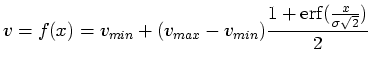$$v = f(x) = v_{min}+(v_{max}-v_{min})\frac{1+\operatorname{erf}(\frac{x}{\sigma \sqrt{2}})}{2}$$ (6)

In its current form, the ideal boundary gets its characteristic shape from the $\operatorname {erf}()$ function. We define this important function and plot it in Figure 5.1.

$$\operatorname{erf}(x) \equiv \frac{2}{\sqrt{\pi}} \int_{0}^{x}e^{-t^2}~dt$$ (7)

Figure 5.1: The error function, $\operatorname {erf}()$

Note in Figure 5.1 that since $\operatorname {erf}()$ is centered around the origin, the boundary function $f(x)$ is also centered around where position $x$ is zero. There are two essential differences between $f(x)$ and $\operatorname{erf}(x)$. First, in $f(x)$ the argument of $\operatorname {erf}()$ is scaled by $1/\sigma \sqrt{2}$. The $\sigma$ parameter controls the thickness, or spread, of the boundary. For large $\sigma$, the argument of $\operatorname {erf}()$ is reduced, and the boundary is stretched out more. The boundary is much narrower and sharper with a small $\sigma$. Second, $\operatorname {erf}()$'s range has been shifted and scaled so that the range of $f(x)$ is between $v_{min}$ and $v_{max}$. As $x$ approaches negative infinity, $\operatorname{erf}(\frac{x}{\sigma \sqrt{2}})$ approaches $-1$, and thus $f(x)$ approaches $v_{min}$. Conversely, as $x$ approaches positive infinity, $f(x)$ approaches $v_{max}$. At $x=0$, the middle of the boundary, $f(x)$ is half-way between $v_{min}$ and $v_{max}$.

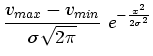
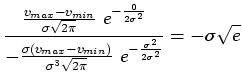
The first and second derivatives of $f$ are as follows:

$$f'(x) = \frac{v_{max}-v_{min}}{\sigma \sqrt{2\pi}}~e^{-\frac{x^2}{2\sigma ^2}}$$ (8)

$$f''(x) = -\frac{x(v_{max}-v_{min})}{\sigma ^3\sqrt{2\pi}}~e^{-\frac{x^2}{2\sigma ^2}}$$ (9)

Our choice of boundary parameterization means that $f'(x)$ is a normalized Gaussian, with $\sigma$ being the usual standard deviation.

 

Figure 5.2: Relationship between thickness and the boundary function. The thickness of material boundaries is defined to be $2\sigma$, which extends from one extremum in $f''$ to the other. The middle of the boundary is defined to be where $x=0$.

Since the Gaussian has inflection points at $\pm\sigma$, this is where $f''(x)$ attains its extrema. The same positions can serve as (somewhat artificial) delimiters for the extent of the boundary. We define the ``thickness'' of the boundary to be $2\sigma$. Figure 5.2 shows how the the definition of thickness roughly accounts for the region in which the data value transitions between the values on either side of the boundary.

The equations for $f'(x)$ (Equation 5.3) and $f''(x)$ (Equation 5.4) look very similar because of the special derivative properties of $e^x$. In fact, the only difference between $f'(x)$ and $f''(x)$ is a scaling factor $\frac{1}{-\sigma ^2}$ and the position $x$:

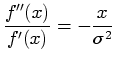$$\frac{f''(x)}{f'(x)} = -\frac{x}{\sigma ^2}$$ (10)

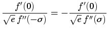
This is intriguing because it means there is a way to infer the position $x$ along a boundary knowing just $\sigma$ and the first and second derivatives. $\sigma$ can be recovered if the extremal values of $f'(x)$ and $f''(x)$ are known. Recall from Figure 5.2 that $f'(x)$ has its maximum at 0, and that $f''(x)$ has a maximum at $-\sigma$ and a minimum at $\sigma$. This gives us two different ways of calculating $\sigma$.

$$\frac{f'(0)}{f''(-\sigma )} = \frac{\frac{v_{max}-v_{min}}{\sigma \sqrt{2\pi}}~e^{-\frac{0}{2\s... ...}{\sigma ^3\sqrt{2\pi}}~e^{-\frac{(-\sigma )^2}{2\sigma ^2}}} = \sigma \sqrt{e}$$

$$\frac{f'(0)}{f''(\sigma )} = \frac{\frac{v_{max}-v_{min}}{\sigma \sqrt{2\pi}}~e^{-\frac{0}{2\s... ...})}{\sigma ^3\sqrt{2\pi}}~e^{-\frac{\sigma ^2}{2\sigma ^2}}} = -\sigma \sqrt{e}$$

$$\Rightarrow \sigma = \frac{f'(0)}{\sqrt{e} \, f''(-\sigma )} = -\frac{f'(0)}{\sqrt{e} \, f''(\sigma )}$$ (11)

Knowing $\sigma$, one can then recover position from $f'(x)$ and $f''(x)$ with Equation 5.5:

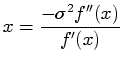$$x = \frac{-\sigma ^2 f''(x)}{f'(x)}$$ (12)

Section 3.4 described the ability to transform the first and second derivatives as functions of position into functions of data value. That transformation takes on special importance in light of Equation 5.7. $f'$ and $f''$ are functions of position in that equation, but there is no reason why they couldn't also be functions of data value. In that case, we would have a way to map from data value back to position along a boundary. Since our goal is to produce an opacity function which makes the middle of boundaries opaque, this information is exactly what is necessary for opacity function generation.

Fortunately, the histogram volume contains that information. The histogram volume was created by recording the position-independent relationship between the data value and its derivatives. In that case, the position that was ``projected out'' in the histogram formation was the $(x,y,z)$ position within the volume. Now, having created the histogram volume, in the next section we will analyze it in order to re-create ``position'' information with Equation 5.7. This time, the ``position'' in question is actually a signed distance to the nearest boundary, which will be extremely helpful in the creation of opacity functions.