Studying $f$, $f'$, and $f''$ in a boundary

Even though the first and second directional derivatives are quantities defined in three dimensions, the significant relationship between them can be reduced to a one dimensional case, because we only care about the value and its derivatives as we move along the gradient direction. Thus, in analyzing the relationship between $f$, $f'$, and $f''$, it suffices to study a one dimensional sampling perpendicular to the surface. Figure 3.4

Figure 3.4: Ideal boundary analysis. The data value and its first and second derivatives are sampled along a short segment which passes through an object boundary

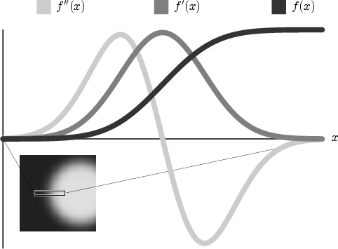analyzes one segment of a slice from the synthetic cylinder dataset. Shown are plots of the data value, and the first and second derivatives, as we move across the cylinder's boundary. The direction of the gradient obviously varies throughout the volume, but the observed relationship between $f$ and its directional derivatives is constant, because the boundary is assumed uniform everywhere. Note that at the mid-point of the boundary, the first derivative is at a maximum, and the second derivative has a zero-crossing. Because of blurring, the boundary is spread over a range of positions, but the maximum in $f'$ and/or the zero-crossing in $f''$ provides a way to define an exact spatial location of a boundary. Indeed, two edge detectors common in computer vision, Canny [Can86] and Marr-Hildreth [MH80], use the $f'$ and $f''$ criteria, respectively, to find edges.