One dimensional masks from reconstruction filters

Figure 4.3 demonstrated the use of a simple mask which was used to measure the first derivative in one dimensional data. This appendix will describe a process which produces masks for measuring derivatives in one dimension, as well as how to generalize one dimensional masks to measure first and second partial derivatives in three dimensions¹⁹.

It was stated in Chapter 4 that reconstruction of a continuous data value function between sample points in the volume dataset is not necessary for measuring any of the quantities needed in the histogram volume creation. Instead, discrete masks can be used to measure the first and second partial derivatives which are needed for the directional derivative calculations. Although we will not need to explicitly reconstruct the data value anywhere, a simple way to derive the necessary masks is through consideration of reconstruction filters and convolution.

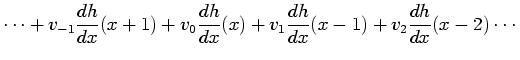
Given a sequence of sampled data points $v_i$, the creation of a continuous function which interpolates smoothly between them starts with a train of delta function spikes at unit intervals, scaled by the original data values:

$$g(x) = \cdots + v_{-1}\delta (x+1) + v_{0}\delta (x) + v_{1}\delta (x-1) + v_{2}\delta (x-2) + \cdots$$ (35)

A continuous reconstructed signal can then be obtained by convolving $g(x)$ with a continuous kernel $h(x)$:

$$(g\star h)(x) = \cdots + v_{-1}h(x+1) + v_{0}h(x) + v_{1}h(x-1) + v_{2}h(x-2) \cdots$$ (36)

Copies of the kernel are effectively placed at each sample point and scaled by the corresponding data value. The first derivative of the reconstructed function is easily computed, by the linearity of taking derivatives:

$${\frac{d(g\star h)}{dx}(x)}$$

$$= \cdots + v_{-1}\frac{dh}{dx}(x+1) + v_{0}\frac{dh}{dx}(x) + v_{1}\frac{dh}{dx}(x-1) + v_{2}\frac{dh}{dx}(x-2) \cdots$$

$$= \cdots + v_{-1}h'(x+1) + v_{0}h'(x) + v_{1}h'(x-1) + v_{2}h'(x-2) \cdots$$

$$= \left[\cdots~v_{-1}~v_{0}~v_{1}~v_{2}~\cdots\right]^T \left[\cdots~h'(x+1)~h'(x)~h'(x-1)~h'(x-2)~\cdots\right]$$ (37)

Equation B.3 defines the infinite sum as the dot product of two vectors, one listing the data values $v_i$, and one containing evaluations of the derivative of the kernel $h$. If the position $x$ where we calculate the derivative of the reconstructed function happens to be an integer $k$, we can express this as:

$${\frac{d(g\star h)}{dx}(k) = }$$

$$\left[\cdots~v_{k-2}~v_{k-1}~v_{k}~v_{k+1}~v_{k+2}~\cdots\right]^T \left[\cdots~h'(2)~h'(1)~h'(0)~h'(-1)~h'(-2)~\cdots\right]$$

Assuming that the reconstruction kernel $h$ has finite support, there can only be a finite number of non-zero values in the vector $\left[\cdots\,\!h'(2)\,h'(1)\,h'(0)\,h'(-1)\,h'(-2)\,\!\cdots\right]$. The finite vector containing all the non-zero values is a mask for measuring the first derivative of regularly sampled data. Since most reconstruction kernels are even functions ( $h(-x) = h(x)$), the mask will have an odd number of values, with $h'(0)$ at the center position. Equation B.4 shows how a mask is used: after centering the mask at the data point of interest ($v_k$), the products between corresponding data and mask values are summed to produce the final measurement.

Given any continuous reconstruction kernel $h(x)$, we can evaluate its first derivative at integer positions to generate a first derivative mask. Of course, the first derivative has to exist at the integer positions in order for this to be valid. As an example, we take the Catmull-Rom cubic spline $c(x)$:

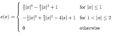$$c(x) = \left\{ \begin{array}{ll} \frac{3}{2}\vert x\vert^3 - \fra... ...{for $1 < \vert x\vert \le 2$} \\ 0 & \mbox{otherwise} \\ \end{array} \right.$$ (39)

One can verify that $c'(x)$ is continuous; evaluating $c'(x)$ at the integers yields:

$$[\cdots~~c'(2)~~c'(1)~~c'(0)~~c'(-1)~~c'(-2)~~\cdots] = [\cdots~~0~-0.5~~0~~0.5~~0~~\cdots]$$ (40)

Thus the Catmull-Rom kernel generates the first derivative mask $[-0.5~~0~~0.5]$.

In the same way that first derivative masks were derived above, masks for measuring the second derivative of regularly sampled data can be created from a kernel $h(x)$:

$$[\cdots~~h''(2)~~h''(1)~~h''(0)~~h''(-1)~~h''(-2)~~\cdots]$$

In this case, the second derivative of the reconstruction kernel must exist at all integer locations for the mask to be valid. For instance, by differentiating $c(x)$ twice, one will find that the Catmull-Rom kernel does not generate a second derivative mask because its second derivative is discontinuous at $\pm 1$ and $\pm 2$.

Footnotes

... dimensions¹⁹

In Chapter 3 we employed an abuse of terminology, using ``first derivative'' for ``first directional derivative along the gradient direction''. In this section we return to the strict usage; ``first derivative'' means the first derivative of a function of one variable (and likewise for a second derivative).