Two common masks and a kernel which generates them

As was noted in Section 4.3, a common mask for measuring the first derivative is $[-0.5~~0~~0.5]$, called the ``central difference'' method. The name arises from the derivative approximation for a function $s(x)$:

$$s'(x) \approx \frac{s(x+d) - s(x-d)}{2d}$$

$$= \frac{1}{2d}s(x+d) - \frac{1}{2d}s(x-d)$$

$$= [s(x-d)~~s(x)~~s(x+d)]^T~[\frac{1}{2d}~~0~-\frac{1}{2d}]$$ (41)

Setting $d=1$ gives the $[-0.5~~0~~0.5]$ mask. In the interests of implementation simplicity and computational speed, this thesis adopts central differences for the first derivative mask. In the context of volume rendering, central differences are often used to calculated the gradient magnitude as part of the shading calculations [LCN98]. There are more sophisticated derivative measurement techniques available [MMMY96], but a thorough exploration of them is tangential to the goal of this thesis.

There is another simple and common mask for our second derivative measurement, $[1~-2~~1]$, sometimes called the ``second central difference'' method. The name arises from the fact that the mask can be derived by twice applying the method of central differences (now with $d=1/2$), as follows:

$$s''(x) \approx s'(x+\frac{1}{2}) - s'(x-\frac{1}{2})$$

$$\approx s(x+1) - s(x) - (s(x) - s(x-1))$$

$$= s(x+1) - 2s(x) + s(x-1)$$

$$= [s(x-1)~~s(x)~~s(x+1)]^T~[1~-2~~1]$$ (42)

This mask does not respond to sequences of constant or linearly changing values. Its result is non-zero only when the sample data point positioned at the middle of the mask is higher or lower than the average of its two neighbors. This thesis uses $[1~-2~~1]$ for the second derivative mask, again in the interests of implementation simplicity and computational speed.

There is an important theoretical question regarding the validity of using these two masks in combination for the histogram volume computation. Recall from Chapter 3 that we traced along an ideal boundary to reveal a characteristic relationship between the data value and its first and second derivatives, as illustrated in Figure 3.8. The point $(f(x),f'(x),f''(x))$ was plotted for each position $x$ along the boundary in order to form the three dimensional curve which indicates the presence of a boundary. For such a case, the boundary function $f(x)$ studied was a continuous function with analytically known derivatives, thus reconstruction was not an issue.

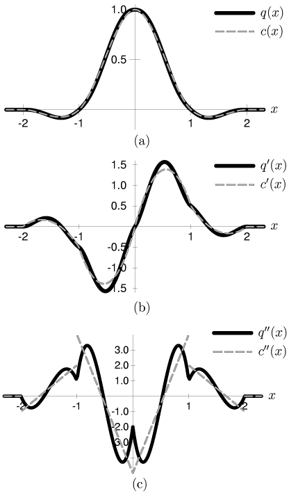
However, when we are measuring derivatives of sampled data with masks, we are implicitly reconstructing the function. That is, the result of using a mask is mathematically equivalent to convolving the sample points with a continuous kernel and analytically finding the derivative of the reconstructed function. Thus, there is a basic incompatibility if there does not exist a reconstruction kernel which can generate both the first and second derivative masks being used. For such a case, the first and second derivatives measures would be based on different reconstructions of the same data. There is no guarantee that the relationship observed in Figure 3.8 will hold if the first and second derivatives are taken from entirely different functions.

It is therefore imperative that we find a reconstruction kernel which generates $[-0.5~~0~~0.5]$ and $[1~-2~~1]$ as its first and second derivative masks, respectively. A piece-wise quintic polynomial kernel $q(x)$ was found which has all the necessary derivative characteristics²⁰:

$$q(x) = \left\{ \begin{array}{ll} 1 - \vert x\vert^2 - \frac{9}{2}... ...{for $1 < \vert x\vert \le 2$} \\ 0 & \mbox{otherwise} \\ \end{array} \right.$$ (43)

The kernel, as well as its first and second derivatives, is plotted in Figure B.1.

Figure B.1: The quintic kernel $q(x)$ and its derivatives. In (a) $q(x)$ is plotted along with the Catmull-Rom kernel $c(x)$ for comparison. The first derivatives of the two kernels are plotted in (b); both have continuous first derivatives, and both generate the $[-0.5~~0~~0.5]$ mask. The second derivatives are plotted in (c); the Catmull-Rom kernel has discontinuous second derivatives, unlike $q(x)$, which generates the $[1~-2~~1]$ second derivative mask.

Although $q(x)$ looks very similar to the Catmull-Rom kernel $c(x)$ (also plotted) the differences become apparent upon taking derivatives, revealing that $q(x)$ is a higher degree polynomial than $c(x)$. Because $q(x)$, unlike $c(x)$, has continuous second derivatives, it can be used to generate a second derivative mask.

This quintic kernel was never implemented in the software for histogram volume generation, because it was never needed for any derivative measurements. Rather, its mere existence provides necessary justification for the approach taken in this thesis. It insures that there is some reconstruction of the sampled data which is consistent with the masks utilized for measuring derivatives. Equation B.3, and its analog for the second derivative, prove that the two masks we have chosen provide exact measures for the first and second derivatives of the data value as a continuous function of position, for the case where the data value was reconstructed with this quintic interpolation kernel.

Footnotes

... characteristics²⁰

The polynomial was found as the solution to a set of differential equations using the Mathematica symbolic math program from Wolfram Research, Champaign, Illinois.